Python Peak Finding - Divide and Conquer

Even simple comparisons can add up to be a performance killer when data gets large enough. A classic divide and conquer approach can really help an algorithm scale with its input.

The Problem

Suppose you have a lump of data, comprising of numbers stored in an array (or Python list). The numbers were not randomly chosen, instead they describe some natural phenomenon. You could plot these numbers on a 2D graph, with each element of the array a new point on the x-axis, and the value of each element as the position on the y-axis. Joining the points up with a line, would show you how the values of the elements vary with respect to their position in the array. Because the numbers in your data are not random, there will be separate regions of the (line) graph that could be considered inclines, peaks and declines. Their could be any number of peaks in this graph, but you have been tasked with creating an algorithm to identify any one of them. For the sake of the algorithm, that will be working on the array (not a graph), a peak is defined as:_ any element that has greater or equal value than that of it’s immediate neighbours_. So, in an array…

[3, 2, 5, 5, 1, 4, 1]

..the 3, both 5’s and the 4 are all peaks. Yes, a peak can be at the start or end of the array, in that case it only has to be larger than its one neighbour. The 5’s form one peak where returning either is acceptable, because they are both greater than a neighbour but equal to the other. The 4 should be clear!

Solution 1 - Iterate The Array

The first way we could solve this is so intuitive, it almost doesn’t need explaining. We simply create an algorithm to check every element of the array, in order, until it finds a peak. Given an input array X, comprised of n elements in positions described by i, we could…

Check if the element at i is larger than or equal to the element at i - 1, if not then increment i and repeat this step.
Check if the element at i is larger than or equal to the element at i + 1, if not then increment i and return to step 1.
If the algorithm gets to here, then return the value at i as a peak.

This algorithm works, and will always work given enough time to check the data. Comparing one value to another is an operation that does (on average) take a constant, small, amount of time. It does still take some time though, however small; no operation comes for free. This isn’t an issue up to a given size of n; on the machine I tried this code on it was able to cope with a “worst case” of 100k elements (i.e. one peak, right at the end of the array). Coping in this case meant returning an answer in 0.04s, your threshold for an acceptable calculation time will vary.

Solution 2 - Divide and Conquer

The second solution vastly reduces the number of comparisons required, effectively “homing in” on a peak by splitting the search space into smaller and smaller pieces. This algorithm is recursive, keeping track of the depth of the call tree in a variable called depth. Each time a new index is required, the offset to it from the current location is calculated by n / 2^depth (if offset = 0, then make offset 1).

Pick the element in the middle of the array as i, depth is 1.
Check if i is larger than or equal to the element at i - 1. If not (i - 1 is larger), then increment depth and calculate the offset. Pick the element at i - offset and repeat this step.
Check if i is larger than or equal to the element at i + 1. If not (i + 1 is larger), then increment depth and calculate the offset. Pick the element at i + offset and go to step 2.
If we get here, then we’ve found a peak.

offset gets smaller with each subsequent call. This ensures that the algorithm “homes in” on a peak, never searching back past an element it has already checked. This solution is able to find a peak at the end of an array with 100k elements in 0.00003s, several factors of 10 quicker than solution 1.

That being said, at 100k elements and lower you could likely get away with solution 1; because not many applications (or any person) will notice the difference in timing. However, scale the input data past 100k elements and solution 1 quickly becomes too slow for most applications. At 100M elements, solution 1 took almost 30s to find the peak compared to just 0.00006s for solution 2; only doubling the calculation time for 1000 times the input size. The reason for this difference in performance is the sheer number of comparisons needed in solution 1.

In this “worst case” input, solution 1 will make comparisons for every element in the array. Solution 1 must therefore make 100M comparisons at minimum. The “divide and conquer” in solution 2 means the function is called 37 times for 100M elements; even with several comparisons each time, the total comparisons made will be in the order of 100’s. Of course, any size array with a peak at the start will work well in solution 1, but it’s always important to consider worst cases. Additionally with 100M elements, solution 2 would still find a “left hand peak” in around 0.00006s; it would make the same number of comparisons, just moving lower (left) in the array each time.

A small Visual Example

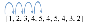
A small visual example may help, if you’re still struggling to picture the second solution. The following shows how how the algorithm moves through indexes using solution 1.

It starts at the beginning, moving to the right until a peak is found. It would find a peak having moved 4 times, making all the comparisons it needed at each element.

This example shows the same array, but with a peak found using algorithm 2.

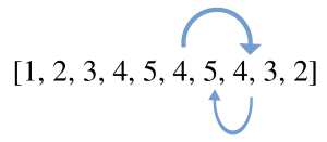
The algorithm starts in the middle with an element equal to 4, which isn’t a peak so depth is incremented from 1 to 2.

The array’s length (n) is 10, so the offset is 10 / 2^2 = 2 (we ignore the .5 using Python integers). The algorithm moves two the right, although left would also be valid. Now the algorithm is on another element of 4 that’s not a peak. It increments depth again; the depth is now 3 so offset is 10 / 2^3 = 1 (this time ignoring the .25). The algorithm moves one to the left, because the element to the right is smaller than 4. This example shows how algorithm 2 “homes in” on a peak, rather than checking every element it can. Now if you mentally scale up the number of elements to the left of the peak, it should be easy to see how algorithm 1 will spend much longer doing comparisons than algorithm 2.